
Jobber custom reports in Google Sheets: five formulas to start with
Build Jobber custom reports in Google Sheets: revenue by month, top clients, overdue invoices, win rate and revenue by service, with how each works.
Jobber's built-in Financial reports, such as Invoices and Aged receivables, each show one fixed view of your data. Its Custom Report Builder is available on the Plus plan, and its reports stay inside Jobber. If you'd rather work in Google Sheets, where you can share a report with a bookkeeper or change it whenever you like, these five formulas answer the questions most service businesses ask first.
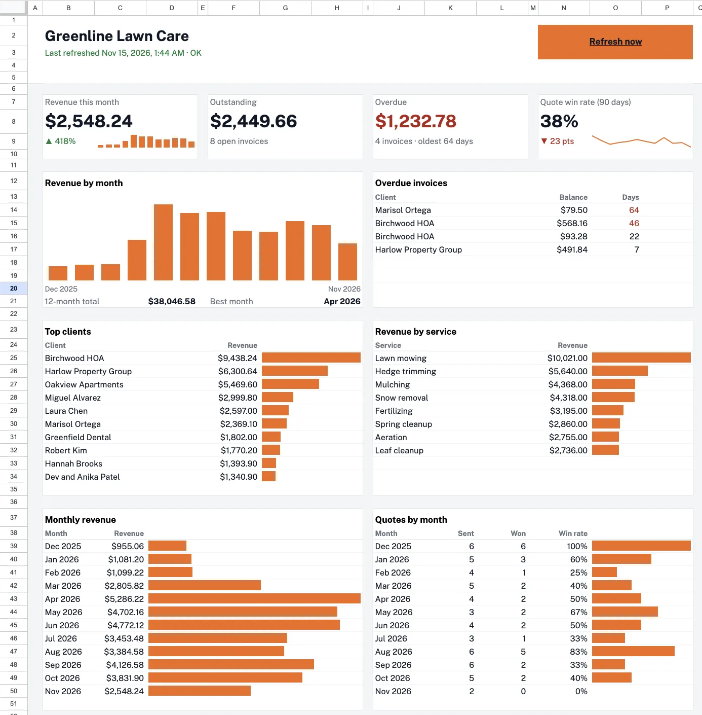
They're written for the tabs SheetVan creates: Invoices, Quotes and Line items. With a CSV export from Jobber the logic is the same, but you'll need to change the column letters to match your file.
Paste each formula into cell A1 of a tab you add yourself. SheetVan rewrites its own data tabs on every refresh but never touches tabs you add, and because the formulas use whole columns, new invoices are included automatically.
Revenue by month
=QUERY(Invoices!A:P, "select year(G), month(G)+1, sum(L) where G is not null and D <> 'Draft' and D <> 'Bad debt' group by year(G), month(G)+1 order by year(G), month(G)+1 label year(G) 'Year', month(G)+1 'Month', sum(L) 'Revenue'", 1)QUERY reads the Invoices tab with its first row as headers; that's the 1 at the end. month() counts from 0, so January comes back as 0, and the +1 turns it into a normal month number. Drafts and bad debt are left out because neither is money you expect to collect.
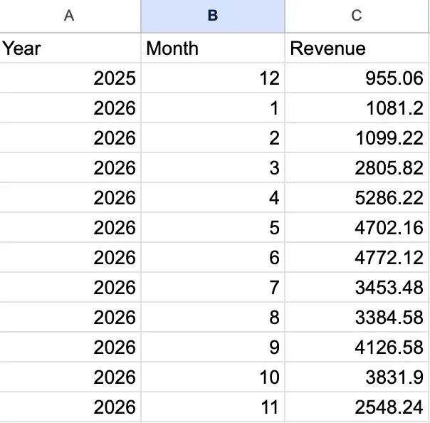
This is revenue invoiced, grouped by issue date. For cash actually received, swap the Issued column (G) for Paid date (I) and Total (L) for Paid (M).
To chart it, select only the Month and Revenue columns, then choose Insert, then Chart. If the Year column is included, Sheets draws the year as its own set of bars next to the revenue.
Top 10 clients
=QUERY(Invoices!A:P, "select F, sum(L) where F is not null and D <> 'Draft' and D <> 'Bad debt' group by F order by sum(L) desc limit 10 label F 'Client', sum(L) 'Revenue'", 1)The same filter as above, grouped by client name and sorted highest first. Two different clients with the same name would be added together; if that's possible in your business, group by the Client ID column instead and look the names up afterwards.
Overdue invoices
=IFERROR(SORT(FILTER({Invoices!F2:F, Invoices!N2:N, TODAY()-Invoices!H2:H}, Invoices!H2:H<TODAY(), Invoices!H2:H<>"", Invoices!N2:N>0, Invoices!D2:D<>"Draft", Invoices!D2:D<>"Bad debt"), 3, FALSE), "Nothing overdue")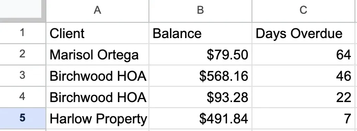
FILTER keeps invoices whose due date has passed and that still have a balance, again skipping drafts and bad debt. That's the same rule the SheetVan Dashboard uses, so the two agree. The third column is days overdue, worked out from TODAY(), so it goes up each day the sheet is opened. When nothing is overdue, FILTER would normally return an error; IFERROR shows "Nothing overdue" instead.
Quote win rate
=IFERROR((COUNTIFS(Quotes!D2:D,"Approved",Quotes!G2:G,"<>")+COUNTIFS(Quotes!D2:D,"Converted",Quotes!G2:G,"<>"))/COUNTIF(Quotes!G2:G,"<>"),"")Only quotes with a Sent date count, on both the top and the bottom of the fraction. A quote approved in person without ever being sent would otherwise push the rate above 100%. Format the cell as a percentage. For a single period, add a date condition on the Sent column to each COUNTIFS. If no quotes have been sent yet, the cell stays blank rather than showing a divide-by-zero error.
Revenue by service
=QUERY('Line items'!A:J, "select F, sum(J) where F is not null and C <> 'Draft' and C <> 'Bad debt' group by F order by sum(J) desc label F 'Service', sum(J) 'Revenue'", 1)This one reads the Line items tab, where each invoice line has its own row, and adds up the line totals for each item. It tells you which services bring in the money, which the invoice totals alone can't show.
The same thing with a pivot table
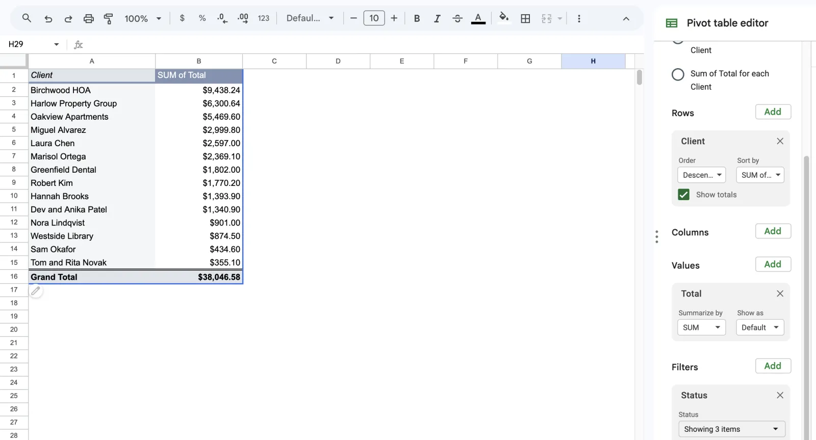
If you'd rather click than type, select a cell in the Invoices tab and choose Insert, then Pivot table. Change the data range to Invoices!A:P so that invoices added later are included; by default Sheets picks a fixed range that stops at the last row. Put Client in Rows and Total in Values, then add a filter on Status to hide Draft and Bad debt, like the formulas above.
Sources
Checked on the date above. Menus in Calendly, Jobber and Zapier change from time to time; if a button has moved, their help pages have the current steps.
SheetVan copies Jobber clients, jobs, invoices, quotes and line items into a Google Sheet every night. How SheetVan works
More guides
Questions or corrections? Email support@sheetvan.com.